Getting performance points with Engauge Digitizer#

In this guide we describe how to load a performance curve using the Engauge Digitizer application.

The first step is to copy the performance map. In the gif below we have an example of a head curve.

After that, go to Engauge -> Edit -> Paste as New.

In the guide wizard we name the curves with the value of each speed:

Note

If you are passing a shaft power curve, you can add the power loss value for each speed with the convention ‘speed, power_loss’:

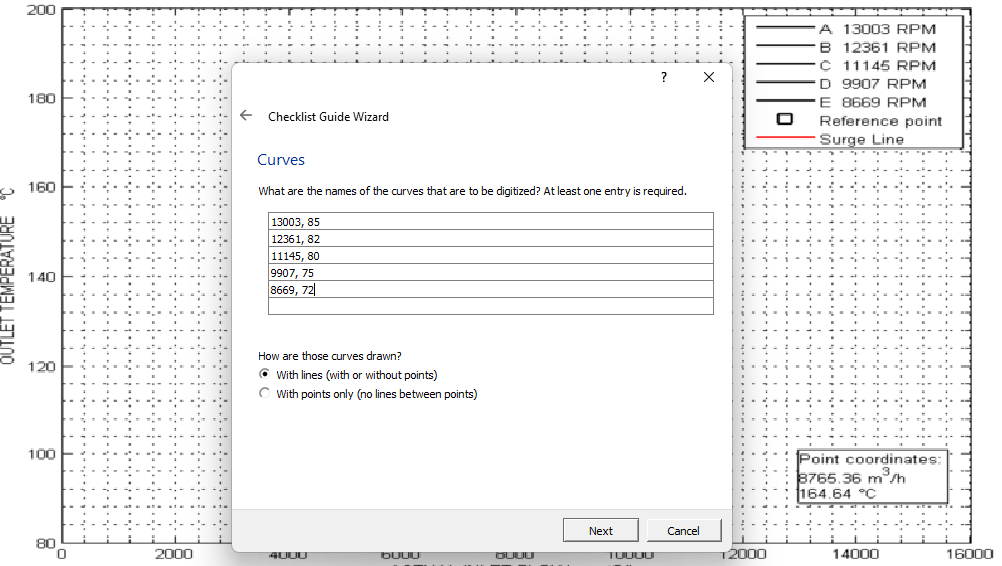
If only one value for power loss is passed, the values for other speeds are calculated based on the ASME PTC 10.

The next step is to select three axis points in the plot:

Now we select a curve and mark the points using the ‘Segment Fill Tool’ or the ‘Curve Point Tool’.

It is recommended to select at least 8 points for each curve to have a good interpolation.

The last step is to configure the export format (Settings -> Export format).

Select ‘Raw Xs and Ys’ and ‘One curve for each line’

After that go to File -> Export and save the .csv file as -head.csv.

Files should be saved with the following convention:

<curve-name>-head.csv
<curve-name>-eff.csv

Do the same steps for the efficiency curve.

After that we can load the data with the following code:

import ccp
from pathlib import Path

data_dir = Path(...)

suc = ccp.State(
    p=Q_(4.08, "bar"),
    T=Q_(33.6, "degC"),
    fluid={
        "METHANE": 58.976,
        "ETHANE": 3.099,
        "PROPANE": 0.6,
        "N-BUTANE": 0.08,
        "I-BUTANE": 0.05,
        "N-PENTANE": 0.01,
        "I-PENTANE": 0.01,
        "NITROGEN": 0.55,
        "HYDROGEN SULFIDE": 0.02,
        "CARBON DIOXIDE": 36.605,
    },
)
imp = ccp.Impeller.load_from_engauge_csv(
    suc=suc,
    curve_name="lp-sec1-caso-a",
    curve_path=data_dir,
    b=Q_(5.7, "mm"),
    D=Q_(550, "mm"),
    head_units="kJ/kg",
    flow_units="m³/h",
    number_of_points=7,
)

In the case above in the data_dir directory we have the files lp-sec1-caso-a-head.csv and lp-sec1-caso-a-eff.csv.