
Straight-Through App Guide#
Table of Contents#
Overview#
The Straight-Through Compressor page is a Streamlit application designed for performance testing and analysis of straight-through centrifugal compressors according to ASME PTC 10 standards.
Key Features#
Multi-gas support: Define up to 6 different gas compositions
Automatic flow calculation: Using orifice plate measurements
Variable speed analysis: Calculate optimal speed to match discharge pressure
Performance curve visualization: Interactive plots with customizable ranges
Data persistence: Save and load complete session states
Getting Started#
Accessing the Application#
Navigate to the CCP application URL
Select “1_straight_through” from the sidebar menu
The main interface will load with expandable sections for data input
Initial Setup#
When starting a new analysis, follow these steps in order:
Define gas compositions
Enter guarantee point data (Data Sheet)
Upload or define performance curves
Input test data
Configure flowrate calculation (if needed)
Run calculations
Interface Layout#
The Straight-Through page consists of several sections:
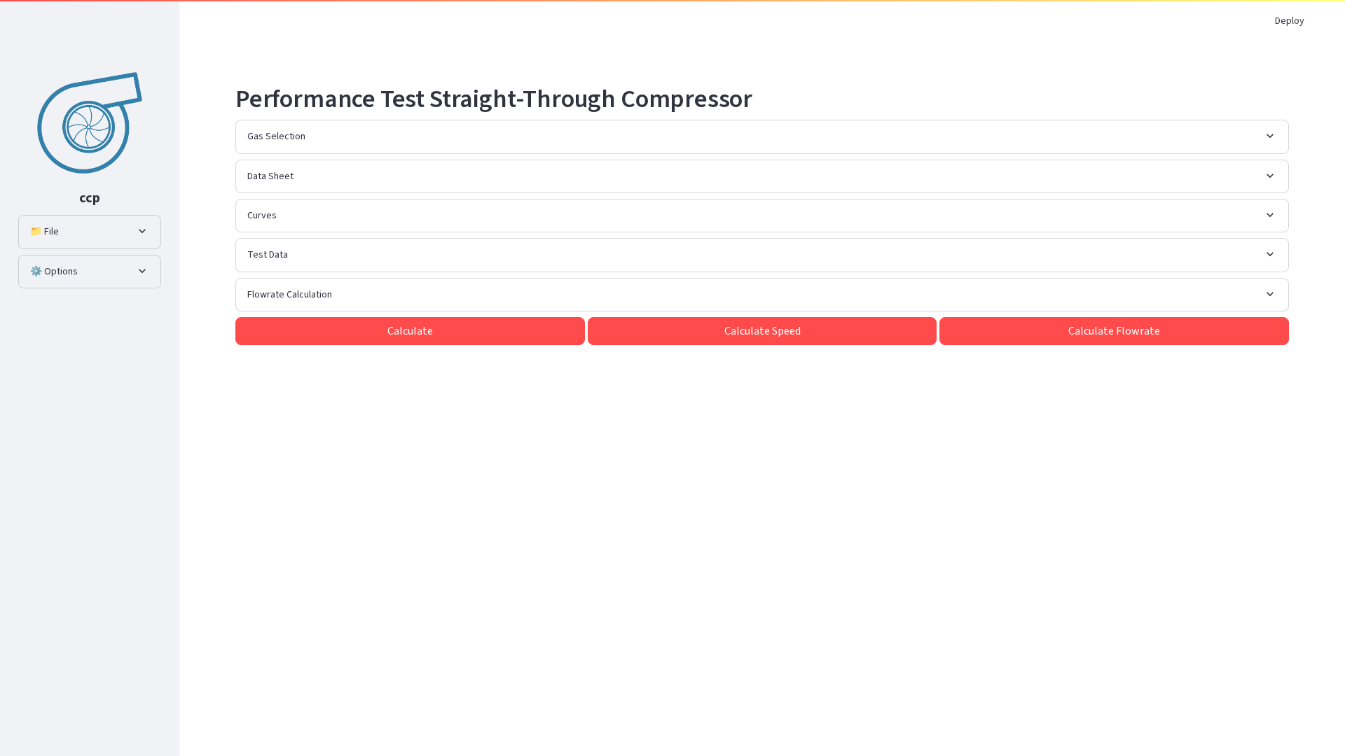
Main interface showing the expandable sections and sidebar options
Main Content Area#
The main area contains expandable sections for different aspects of the analysis:
Gas Selection: Define gas compositions
Data Sheet: Enter guarantee point specifications
Curves: Upload or define performance curves
Test Data: Input actual test measurements
Flowrate Calculation: Calculate flow using orifice measurements
Results: View calculation outputs and plots
Gas Selection#
Defining Gas Compositions#
The Gas Selection section allows you to define up to 6 different gas compositions that can be used throughout the analysis.
For each gas:#
Gas Name: Enter a descriptive name (e.g., “gas_0”, “Natural Gas Mix 1”)
Component Table:
Select components from the dropdown (methane, ethane, etc.)
Enter molar fractions (mol %)
Add/remove rows as needed
Total should sum to 100%
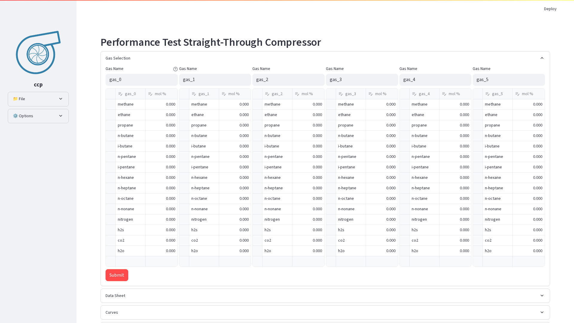
Gas Selection section expanded, showing gas composition definition interface with component tables
Data Sheet Configuration#
The Data Sheet section is where you enter the guarantee point specifications from the compressor data sheet.
Required Parameters:#
Flow Parameters#
Flow: Mass flow (kg/s) or volumetric flow (m³/h)
Units selection: Choose appropriate units from dropdown
Pressure Parameters#
Suction Pressure: Inlet pressure
Discharge Pressure: Outlet pressure
Units: bar, bara, barg, Pa, kPa, MPa, psi, psia
Temperature Parameters#
Suction Temperature: Inlet temperature
Discharge Temperature: Outlet temperature
Units: K, °C, °F, °R
Performance Parameters#
Power: Shaft power requirement
Speed: Rotational speed
Head: Polytropic/isentropic head
Efficiency: Polytropic efficiency
Geometric Parameters#
b (Impeller exit width): Exit width dimension
D (Impeller diameter): Impeller outer diameter
Surface roughness: Internal surface roughness
Casing area: Cross-sectional area for heat transfer
Input Guidelines:#
Select the gas composition for the guarantee point
Choose consistent unit systems
Enter all required values before proceeding
Verify values against original data sheets
Use the help icons (?) for parameter descriptions
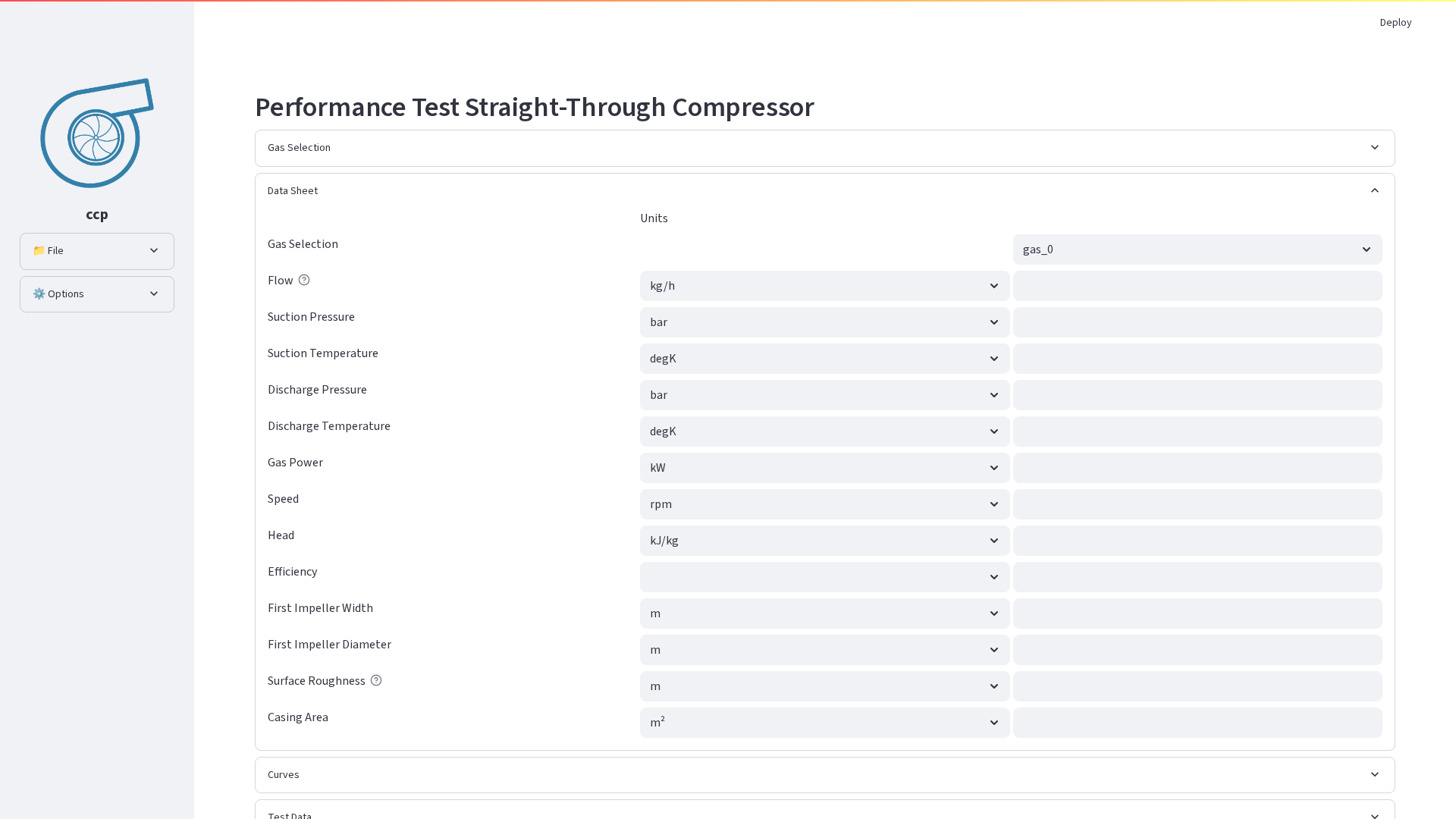
Data Sheet section showing guarantee point parameters including flow, pressure, temperature, and performance specifications
Performance Curves#
Uploading Curve Images#
The Curves section allows you to upload performance curve images and define axis ranges for proper scaling.
For each curve type:#
Head Curve
Efficiency Curve
Discharge Pressure Curve
Power Curve
Steps to Configure:#
Click “Choose File” to upload PNG image of the curve
Define X-axis (flow) range:
Lower limit
Upper limit
Units selection
Define Y-axis range:
Lower limit
Upper limit
Units selection (specific to curve type)
Axis Configuration Tips:#
Match units to your data sheet values
Set ranges equal to the plot ranges
Images will overlay on calculated curves for comparison
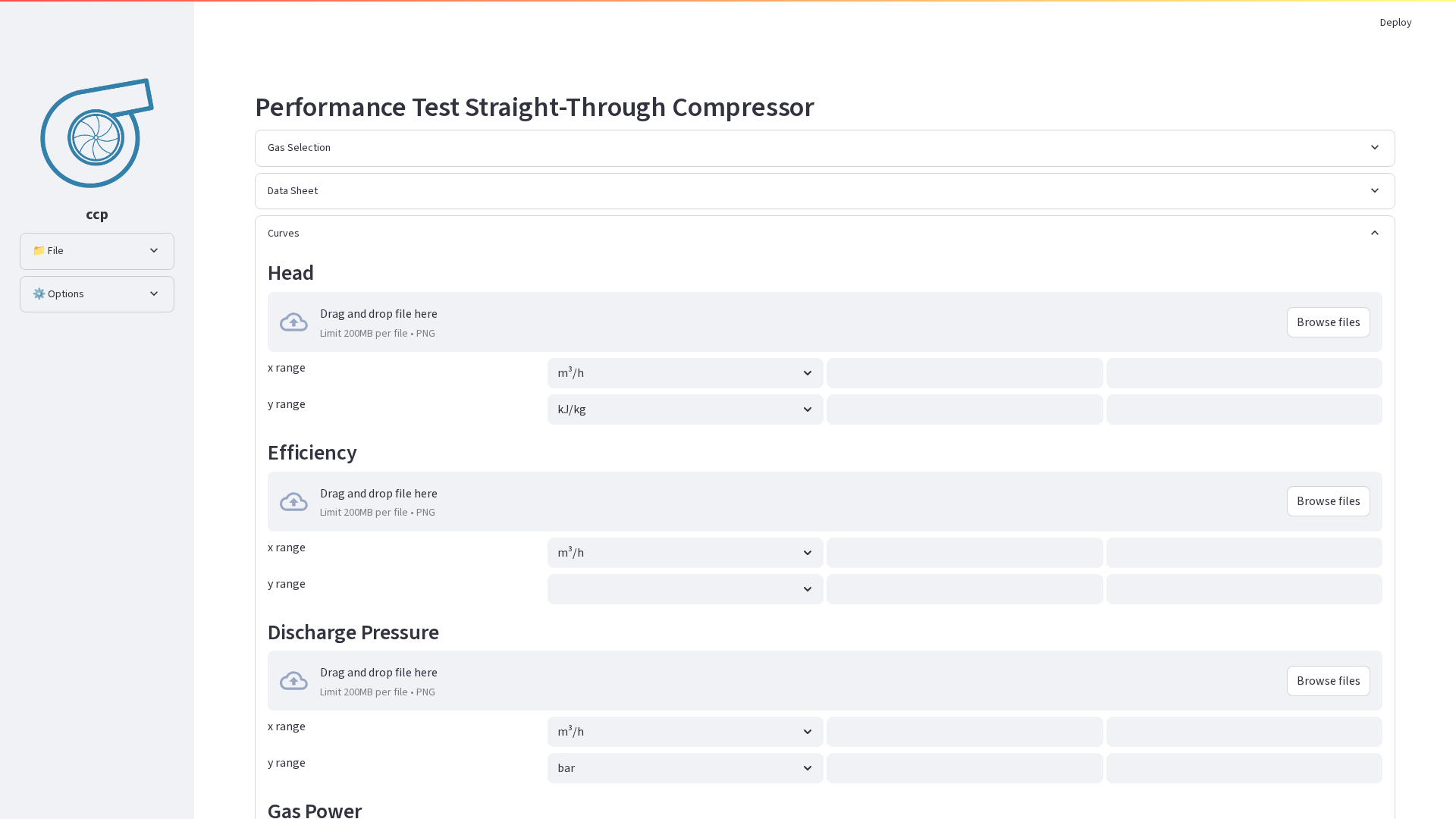
Curves section displaying uploaded performance curve images with axis range configuration options
Test Data Input#
Entering Test Points#
The Test Data section accommodates up to 6 test points for performance evaluation.
For Each Test Point:#
Required Measurements:#
Gas Selection: Choose from defined gases
Flow: Actual measured flow
Suction Pressure: Measured inlet pressure
Suction Temperature: Measured inlet temperature
Discharge Pressure: Measured outlet pressure
Discharge Temperature: Measured outlet temperature
Speed: Actual rotational speed
Optional Measurements:#
Casing Delta T: Temperature difference for heat loss calculation
Balance Line Flow: Leakage flow through balance line
Seal Gas Flow: Flow rate of seal gas (if enabled)
Seal Gas Temperature: Temperature of seal gas
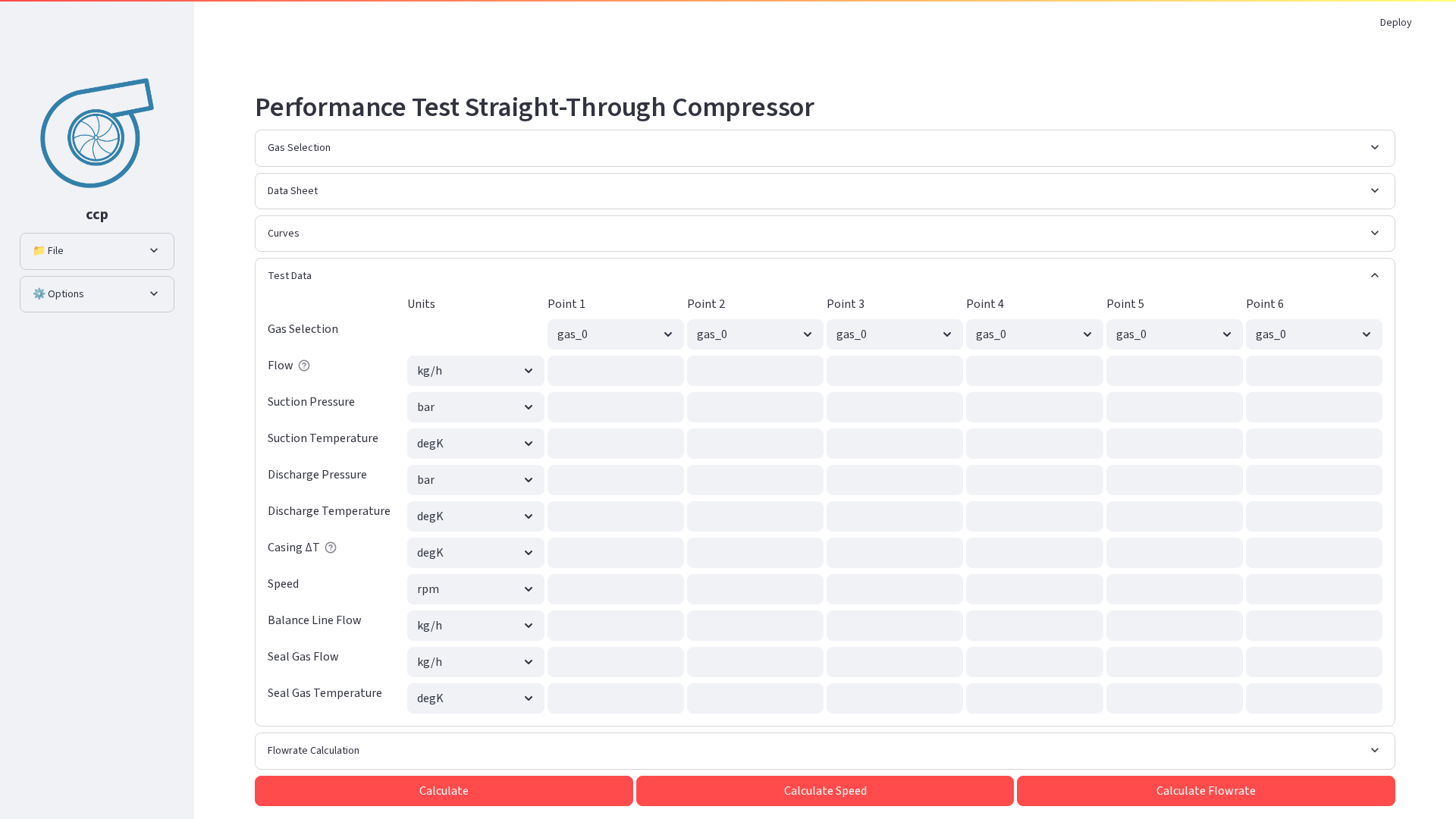
Test Data section showing multiple test points with measured parameters for performance evaluation
Flowrate Calculation#
Using Orifice Plate Measurements#
When direct flow measurement is unavailable, the Flowrate Calculation section computes flow using orifice plate differential pressure measurements.
Required Parameters for Each Point:#
Orifice Geometry:#
Outer Diameter (D): Pipe inner diameter
Inner Diameter (d): Orifice bore diameter
Process Conditions:#
Upstream Pressure: Pressure before orifice
Upstream Temperature: Temperature before orifice
Pressure Drop: Differential pressure across orifice
Configuration:#
Tappings Type:
Flange taps
Corner taps
D and D/2 taps
Gas Selection: Choose gas composition
Calculation Process:#
Enter all orifice parameters
Click “Calculate Flowrate” button
Calculated mass flow appears in the last row
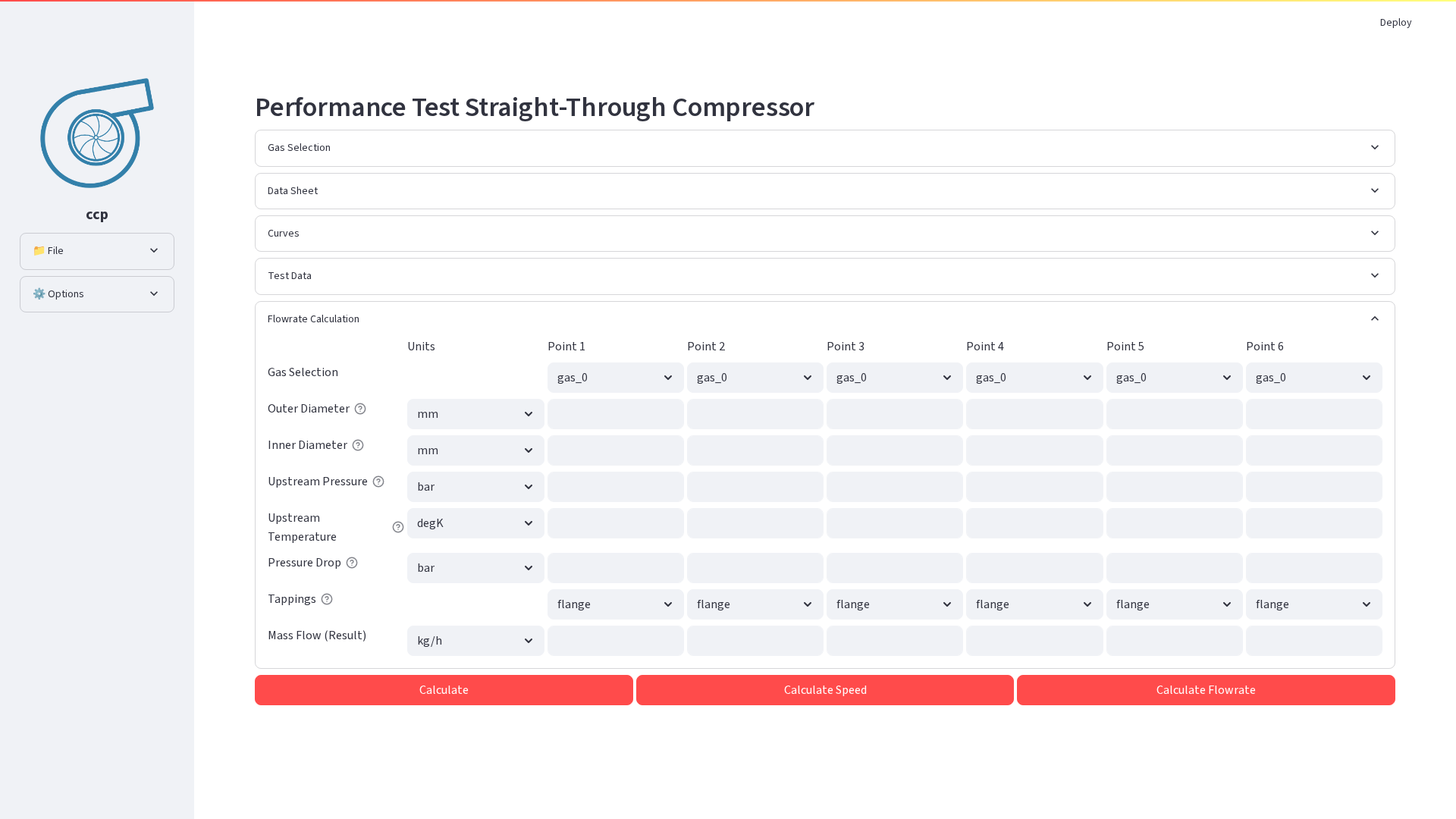
Flowrate Calculation section with orifice plate parameters and differential pressure measurements for flow computation
Running Calculations#
Calculation Options#
Three calculation modes are available:
1. Standard Calculate#
Purpose: Analyze performance at data sheet speed
Process:
Converts test points to guarantee conditions
Applies Reynolds corrections
Generates performance comparison
2. Calculate Speed#
Purpose: Find speed to match discharge pressure
Process:
Iteratively adjusts speed
Matches test discharge pressure to guarantee
Useful for variable speed drives
Execution Steps:#
Verify all required data is entered
Select appropriate calculation mode
Click the corresponding button
Monitor progress bar
Review warnings/errors if any
Examine results section
Understanding Results#
Results Table#
The results section displays a comprehensive comparison table with the following parameters:
Flow Coefficients:#
φt: Test flow coefficient
φt/φsp: Ratio to guarantee point
Volume Ratios:#
vi/vd: Volume ratio
(vi/vd)t/(vi/vd)sp: Volume ratio comparison
Similarity Parameters:#
Macht: Test Mach number
Macht - Machsp: Mach number difference
Ret: Test Reynolds number
Ret/Resp: Reynolds number ratio
Performance Parameters:#
pdconv: Converted discharge pressure
Headconv: Converted head
Qconv: Converted flow rate
Wconv: Converted power
Effconv: Converted efficiency
Color Coding:#
Green highlight: Within acceptable limits
Red highlight: Outside acceptable limits
Acceptance Criteria:#
Mach difference: ±0.05
Reynolds ratio: 0.95-1.05
Volume ratio: 0.95-1.05
Power ratio: <1.04 (variable speed) or <1.07 (fixed speed)
[Screenshot placeholder: Results table with color-coded values]
Performance Plots#
Four interactive plots visualize the performance:
1. Head vs Flow#
Shows test curve and guarantee point
Converted performance curve
Interactive zoom and pan
2. Efficiency vs Flow#
Polytropic efficiency curve
Test points and interpolation
Guarantee point marker
3. Discharge Pressure vs Flow#
Pressure rise characteristics
Operating point indication
Background curve image (if uploaded)
4. Power vs Flow#
Shaft power requirements
Speed-corrected values
Power limit indicators
Plot Features:#
Interactive: Zoom, pan, hover for values
Legends: Click to show/hide traces
Export: Save as PNG or SVG
Background: Original curves overlay
[Screenshot placeholder: Four performance plots arranged in grid]
Additional Visualizations#
Mach Number Plot#
Shows Mach number variation
Acceptable range indication
Critical Mach limit
Reynolds Number Plot#
Reynolds number comparison
Correction factor visualization
Valid range highlighting
File Management#
Saving Sessions#
Save Current Work:#
Enter session name in sidebar
Click “Save” button
File saves as
[session_name].ccp
Save As:#
Click “Save As” button
Download dialog appears
Choose location and filename
Session File Contents:#
All entered data
Gas compositions
Uploaded curves
Calculation results
Plot configurations
Loading Sessions#
Open Saved File:#
Click “Open File” in sidebar
Select
.ccpfileClick “Load” button
All data restores automatically
File Format:#
Compressed ZIP archive
Contains JSON data and images
Version controlled for compatibility
Portable between installations
Example Workflow#
You can find some example files inside ccp/app folder.